Definition : Regression Analysis

Regression analysis models the relationship between one or more response variables (also called dependent variables, explained variables, predicted variables, or regressands) (usually named Y), and the predictors (also called independent variables, explanatory variables, control variables, or regressors,) usually named X1,...,Xp).

If there is more than one response variable, we speak of multivariate regression.

Examples
To illustrate the various goals of regression, we will give three examples.

Prediction of future observations

The following data set gives the average heights and weights for American women aged 30-39 (source: The World Almanac and Book of Facts, 1975).
Height (in) 58 59 60 61 62 63 64 65 66 67 68 69 70 71 72
Weight (lbs)115 117 120 123 126 129 132 135 139 142 146 150 154 159 164

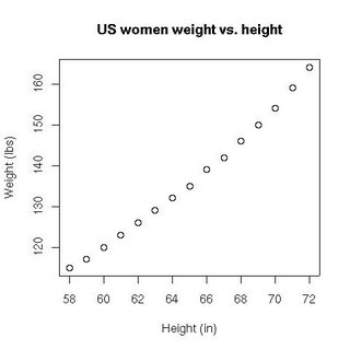
We would like to see how the weight of these women depends on their height. We are therefore looking for a function η such that , where Y is the weight of the women and X their height. Intuitively, we can guess that if the women's proportions are constant and their density too, then the weight of the women must depend on the cube of their height. A plot of the data set confirms this supposition:




_______________________________________________________

X will denote the vector containing all the measured heights
((X=(58,59...)) and (Y= (115,117,120)) is the vector containing all measured weights. We can suppose the heights of the women are independent from each other and have constant variance, which means the Gauss-Markov assumptions hold. We can therefore use the least-squares estimator, i.e. we are looking for coefficients θ0,θ1 and θ2 satisfying as well as possible (in the sense of the least-squares estimator) the equation:




Geometrically, what we will be doing is an orthogonal projection of Y on the subspace generated by the variables 1,X and X3. The matrix X is constructed simply by putting a first column of 1's (the constant term in the model) a column with the original values (the X in the model) and a third column with these values cubed (X3). The realization of this matrix (i.e. for the data at hand) can be written:
1 x x3
1 58 195112
1 59 205379
1 60 216000
1 61 226981
1 62 238328
1 63 250047
1 64 262144
1 65 274625
1 66 287496
1 67 300763
1 68 314432
1 69 328509
1 70 343000
1 71 357911
1 72 373248



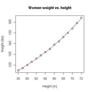
The matrix (sometimes called "information matrix" or "dispersion matrix") is: Vector is therefore: hence A plot of this function shows that it lies quite closely to the data set:

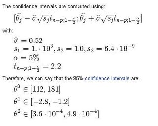
The confidence intervals are computed using:

with: